By scale
topographic maps are divided into:
- small scale (1:1 000 000 - 1:500 000);
- medium scale (1:200 000 - 1:100 000);
- large scale(1:50,000 and larger).
Scale maps 1:25,000 – 1:100,000 are intended for the work of commanders and staffs in the organization, conduct of combat and command and control of troops in combat. They are most widely used as working cards in the tactical level of command and control. They study and evaluate the terrain in preparation for and during hostilities, determine the coordinates of the combat positions of missile forces and artillery, as well as the coordinates of targets, make measurements and calculations in the design and construction of military engineering structures and other objects.
Map scale 1:25 000 used in the troops for a detailed study of the most important lines and areas of the terrain when forcing water barriers, landing, etc.
Map scale 1:50 000 it is used mainly in defense, and in the offensive - mainly when breaking through enemy defenses, forcing water barriers, landing air and sea assault forces, as well as in battles for settlements.
When operating in large settlements, commanders and headquarters can be issued city plans in addition to maps scale 1:10,000 or 1:25,000. They are intended for studying cities and approaches to them, for orientation inside the city, target designation and command and control of troops during the battle for the city. To this end, the plans indicate the names of streets, numbers of quarters and the most important objects of the city with their quantitative and qualitative characteristics.
Maps of scales 1:200,000 and 1:500,000 are intended for the study and evaluation of the terrain in the planning and preparation of operations, for command and control of troops in the course of operations and planning of troop movements. A map at a scale of 1:500,000 is also used by front-line aviation as a flight map.
Map scale 1:200 000 especially convenient as a road, because. visually and sufficiently complete for orientation on the terrain displays the road network and characterizes its suitability for the movement of vehicles and military equipment. Using this map, you can study and evaluate the road network and the general nature of the relief, water lines, forests, and large settlements. This is helped by information about the area, placed on the back of the map sheets. References contain in a generalized and systematized form the necessary additional information about the nature of the area and its individual most important objects that cannot be displayed on the map itself.
In all command and staff instances from the battalion and above, a map at a scale of 1:200,000 is used to navigate the terrain when making marches. In motorized rifle, tank units and formations during the offensive, especially when pursuing the enemy, it is used as the main map.
Map scale 1:1 000 000 is used by headquarters to study the physical and geographical conditions of vast territories and for general, approximate calculations to ensure the combat operations of troops when planning operations.
Fig.1 Ellipse and its elements.
The dimensions of any ellipsoid of revolution are characterized by the major a and minor b semiaxes. Attitude (a - b) / a called
ellipsoid compression. An ellipsoid of revolution has a mathematically correct surface formed by rotating an ellipse about its minor axis. The deviations in height of points on the surface of the geoid from the surface of the ellipsoid closest to it in size are characterized by an average value of about 50 m and do not exceed 150 m. Compared with the dimensions of the Earth, such discrepancies are so insignificant that in practice the shape of the Earth is mistaken for an ellipsoid. An ellipsoid that characterizes the shape and size of the Earth is called earth ellipsoid.
Establishing the dimensions of the earth's ellipsoid, which is closest in shape and size to the actual figure of the Earth, is of great scientific, theoretical and practical importance. This is important for creating accurate topographic maps. If the dimensions of the earth's ellipsoid are set incorrectly, this will lead to incorrect calculations when projecting onto its surface (and, consequently, when depicting on maps) all line lengths and area sizes compared to their actual sizes on the level surface of the Earth. The dimensions of the earth's ellipsoid at different times were determined by many scientists based on the materials of degree measurements. Some of them are shown in Table 1:
Table 1
In the USA, Canada, Mexico, France, when creating maps, they use the dimensions of the Clark ellipsoid, in Finland and some other countries - the dimensions of the Hayford ellipsoid, in Austria - the dimensions of the Bessel ellipsoid, in the USSR and a number of socialist countries - the dimensions of the Krasovsky ellipsoid.
When solving some practical problems, when high accuracy is not required, the figure of the Earth is taken as a sphere, the surface of which (about 510 million km2) is equal to the surface of an ellipsoid of the accepted dimensions. The radius of such a ball, calculated from the elements of the Krasovsky ellipsoid, is 6371 116 m or rounded 6371 km.
Horizontal laying. When depicting the physical surface of the Earth on a map (plane), it is first projected with plumb lines onto a level surface (Fig. 2), and then, according to certain rules, this image is deployed onto a plane.

Fig.2 Projection of the physical surface of the Earth on a level surface.
When depicting a small section of the earth's surface, the corresponding section of the level surface is taken as a horizontal plane and, having projected this section on it, a topographic plan of the area is obtained. The geometric essence of such an image is as follows. If from each point of any straight line AB (Fig. 3), arbitrarily located in space, we lower the perpendicular to the horizontal plane P (the plane of projections), then the points of intersection of the perpendiculars with the plane will form the straight line ab, which will be the planned image of the straight line AB. The image in terms of points and lines of the earth's surface is called their horizontal spacing or horizontal projection.
In the case when the projected line is horizontal, its image in plan is equal to the length of the line itself. If the projected straight line is inclined, then its horizontal distance is always shorter than its length and decreases with increasing angle of inclination. The horizontal span of a vertical line represents a point.

Fig.3 Horizontal spacing (image in plan) of a point, straight, broken and curved lines.
When creating a map, it is applied on a given scale, that is, with a certain decrease, horizontal laying of all points of the terrain, lines, contours, projecting them onto the dropped surface of the Earth, which is taken as a horizontal plane within the map sheet. On the ground, all lines are usually inclined, which means that their horizontal spans are always shorter than the lines themselves.
The essence of cartographic projections. It is impossible to unfold a spherical surface on a plane without gaps and folds, that is, its planned image on a plane cannot be represented without distortion, with a complete geometric similarity of all its outlines. Full similarity of the outlines of islands, continents and various objects projected onto a level surface can be achieved only on a ball (globe). The image of the Earth's surface on a ball (globe) has equal scale, equal angle and equal area.
These geometric properties cannot be stored completely on the map at the same time. A geographic grid built on a plane, depicting meridians and parallels, will have certain distortions, so the images of all objects on the earth's surface will be distorted. The nature and extent of distortions depend on the method of constructing the cartographic grid, on the basis of which the map is compiled.
The display of the surface of an ellipsoid or ball on a plane is called a map projection. There are different types of cartographic projections. Each of them corresponds to a certain cartographic grid and its inherent distortions. In one type of projection, the dimensions of areas are distorted, in another - angles, in the third - areas and angles. In this case, in all projections, without exception, the lengths of the lines are distorted.
Map projections classify by the nature of distortions, the type of image of meridians and parallels (geographic grid) and some other features.
According to the nature of the distortion the following map projections:
- equiangular, maintaining equality of angles between directions on the map and in kind. Figure 4 shows a map of the world, on which the cartographic grid retains the property of equiangularity. The similarity of corners is preserved on the map, but the sizes of areas are distorted. For example, the areas of Greenland and Africa on the map are almost the same, but in reality the area of Africa is about 15 times the area of Greenland.

Fig.4 Map of the world in a conformal projection.
- equal, preserving the proportionality of the areas on the map to the corresponding areas on the earth's ellipsoid. Figure 5 shows a map of the world compiled in an equal area projection. The proportionality of all areas is preserved on it, but the similarity of the figures is distorted, that is, there is no equiangularity. The mutual perpendicularity of the meridians and parallels on such a map is preserved only along the middle meridian.

Fig.5 Map of the world in equal area projection.
- equidistant, maintaining the constancy of the scale in any direction;
- arbitrary, preserving neither the equality of angles, nor the proportionality of areas, nor the constancy of scale. The meaning of the use of arbitrary projections lies in a more uniform distribution of distortions on the map and the convenience of solving some practical problems.
By the appearance of the image of the grid of meridians and parallels map projections are divided into conical, cylindrical, azimuthal, etc. Moreover, within each of these groups there can be projections of different nature of distortion (equiangular, equal-area, etc.).
The geometric essence of conic and cylindrical projections lies in the fact that the grid of meridians and parallels is projected onto the lateral surface of a cone or cylinder with the subsequent deployment of these surfaces into a plane. The geometric essence of azimuth projections is that the grid of meridians and parallels is projected onto a plane tangent to the ball at one of the poles or secant along some parallel.
map projection, The most suitable in terms of the nature, magnitude and distribution of distortions for a particular map is chosen depending on the purpose, content of the map, as well as on the size, configuration and geographical location of the mapped area. Thanks to the cartographic grid, all distortions, no matter how great they may be, do not in themselves affect the accuracy of determining the geographical position (coordinates) of the objects depicted on the map. At the same time, the cartographic grid, being a graphic expression of the projection, makes it possible to take into account the nature, magnitude and distribution of distortions when measuring on a map. Therefore, any geographical map is a mathematically defined image of the earth's surface.
Fig.6 Division of the Earth's surface into six-degree zones.
To imagine how the image of zones is obtained on a plane, imagine a cylinder that touches the axial meridian of one of the zones of the globe (Fig. 7). According to the laws of mathematics, we project the zone onto the lateral surface of the cylinder so that the property of the equiangularity of the image is preserved (the equality of all angles on the surface of the cylinder to their magnitude on the globe). Then we project all other zones, one next to the other, onto the side surface of the cylinder. Further cutting the cylinder along the generatrix AA1 or BB1 and turning its lateral surface into a plane, we obtain an image of the earth's surface on a plane in the form of separate zones (Fig. 8).

Fig.7 Zone projection onto the cylinder.

Fig.8 The image of the zones of the earth's ellipsoid on the plane.
The axial meridian and the equator of each zone are depicted as straight lines perpendicular to each other. All axial meridians of the zones are depicted without length distortion and maintain the scale throughout their entire length. The remaining meridians in each zone are depicted in the projection as curved lines, so they are longer than the axial meridian, that is, they are distorted. All parallels are also shown as curved lines with some distortion. Line length distortions increase with distance from the central meridian to the east or west and become greatest at the edges of the zone, reaching a value of the order of 1/1000 of the line length measured on the map. For example, if along the axial meridian, where there is no distortion, the scale is 500 m in 1 cm, then at the edge of the zone it will be 499.5 m in 1 cm.
It follows that topographic maps are distorted and have a variable scale. However, these distortions when measured on a map are very small, and therefore it is believed that the scale of any topographic map for all its sections is practically constant.
Thanks to single projection all our topographic maps are connected with a system of flat rectangular coordinates, in which the position of geodetic points is determined, and this allows us to obtain the coordinates of points in the same system both on the map and when measuring on the ground.
2). Graphing and nomenclature
The system for dividing a map into separate sheets is called map layout, and the system of designation (numbering) of sheets - their nomenclature.
The division of topographic maps into separate sheets by lines of meridians and parallels is convenient because the frames of the sheets accurately indicate the position on the earth's ellipsoid of the area depicted on this sheet, and its orientation relative to the sides of the horizon.
Standard card sheet sizes different scales are shown in table 1:
Table 1
Layout scheme 1:1,000,000 scale maps are shown in Figure 1.

Fig.1. Layout and nomenclature of map sheets at a scale of 1:1,000,000.
The principle of laying out maps of other scales (larger ones) is shown in Fig. 2.3.

Fig.2. Location, numbering order and designation of map sheets
scales 1:50,000 - 1:500,000 on a sheet of a millionth map.

Fig.3. Layout and nomenclature of sheets of maps at a scale of 1:50,000 and 1:25,000.
From Table 1 and these figures, it can be seen that a sheet of a millionth map corresponds to an integer number of sheets of other scales, a multiple of four - 4 sheets of a map of a scale of 1:500,000, 36 sheets of a map of a scale of 1:200,000, 144 sheets of a scale of 1:100,000, etc. d.
In accordance with this, the nomenclature of sheets was established, which is the same for topographic maps of all scales. The nomenclature of each sheet is indicated above the north side of its frame.
table 2
| Types of cards | map scale | Card types | The order of formation of the map sheet | Map sheet formation scheme | Map sheet size | Nomenclature example |
| Operational | 1:1000000 | small scale | division of the earth's ellipsoid by parallels, meridians | 6° 4° | 4° × 6° | C-3 |
| 1:500000 | dividing a sheet of a millionth card into 4 parts | A B C D | 2° × 3° | S-3-B | ||
| 1:200000 | Medium scale | division of a sheet of a millionth card into 36 parts | XVI | 40" × 1° | С-3-XVI | |
| Tactical | 1:100000 | division of a sheet of a million card into 144 parts | 20" × 30" | C-3-56 | ||
| 1:50 000 | large scale | division of the map sheet M. 1: 100 000 into 4 parts | A B C D | 10" × 15" | C-3-56-A | |
| 1:25 000 | division of the card sheet M. 1:50 000 into 4 parts | a B C D | 5" × 7" 30" | C-3-56-A-b | ||
| 1:10 000 | division of the map sheet M. 1:25 000 into 4 parts | 1 2 3 4 | 2" 30" × 3" 45" | C-3-56-A-b-4 |
To select the necessary map sheets for a particular area and to quickly determine their nomenclature, there are so-called prefabricated map tables (Fig. 4). They are small-scale diagrams, divided by meridians and parallels into cells corresponding to ordinary map sheets at a scale of 1:100,000, indicating their serial numbering within the sheets of a millionth map.

Fig. 4 Clipping from the map table at a scale of 1:100,000.
An extract of the nomenclature of the required sheets is carried out from left to right and from top to bottom. For example, if you need to get maps in scales of 1:100,000 and 1:50,000, for example, for the Mozyr-Loev region (in Fig. 4 this region is shaded), then the list of nomenclatures of these sheets in the application for maps will look like this:
| 1:100 000 | 1:50 000 |
| N-35-143, 144; | N-35-143-A, B, C, D; M-35-11-A, B, C, D; |
| N-36-133, 134; | N-35-144-A, B, C, D; M-35-12-A, B, C, D; |
| M-35-11, 12; | N-36-133-A, B, C, D; M-36-1-A, B, C, D; |
| M-36-1, 2; | N-36-134-A, B, C, D; M-36- 2-A, B, C, D. |
Fig.1 Plumb line deviation from the normal at point M.
Thus, geographic coordinates are a generalized concept of astronomical and geodetic coordinates, when the deviation of the plumb line is not taken into account.
Astronomical coordinates. astronomical latitude point M (Fig. 2) is called the angle (phi) (Fig. 1), formed by a plumb line at a given point and a plane perpendicular to the axis of rotation of the Earth. Astronomical longitude point M is called the dihedral angle (lamda) between the planes of the astronomical meridian of the given point and the initial (zero) astronomical meridian. The astronomical meridian of a point is a trace of the section of the earth's surface by a plane passing through the direction of the plumb line at this point parallel to the axis of rotation of the Earth. In sea and air navigation during astronomical observations, the difference in longitudes of two points is determined by the difference in time at the same points. Every 15° in longitude corresponds to 1 hour, since the rotation of the Earth by 360° takes 24 hours. Therefore, the meridians on navigation maps are signed not only in degrees, but also in hours. For example, the meridian of the point 45 ° 30 "East longitude in time will have a value of 3 hours 02 minutes. Thus, knowing the longitude of two points, it is easy to determine the difference in local time at these points.

Fig.2 Astronomical coordinates.
Geodetic coordinates. Geodetic latitude point A (Fig. 3) is called the angle B formed by the normal to the surface of the earth's ellipsoid at a given point and the plane of the equator. Latitude is measured along the meridian on both sides of the equator and can take values from 0 to 90°. The latitudes of points located north of the equator are called northern (positive), and to the south - southern (negative).
Geodetic longitude point A is the dihedral angle L between the planes of the geodesic meridian of the given point and the initial (zero) geodesic meridian. The plane of the geodesic meridian passes through the normal to the surface of the earth's ellipsoid at a given point parallel to its minor axis. The longitudes of the points are measured from the initial meridian to the east and west and are called east and west, respectively. They are counted from 0 to 180° in each direction.

Fig.3 Geodetic coordinates.
2).Determination by map
Determination of geographical (geodesic) coordinates of points on the map. The internal frames of topographic maps are segments of parallels and meridians. Their latitude and longitude are signed at the corners of each sheet of the map. On maps of the Western Hemisphere, in the northwestern corner of the frame of each sheet, to the right of the longitude of the meridian, the inscription is placed: "West of Greenwich."
On maps of scales 1:25000-1:200000, the sides of the frames are divided into segments equal to V. These segments are shaded through one and divided by points (except for the map at a scale of 1:200,000) into parts of 10 ". On each sheet of the map at a scale of 1:50000 and 1:100000 show, in addition, the intersection of the middle meridian and parallels with digitization in degrees and minutes, and along the inner frame - outputs of minute divisions with strokes 2-3 mm long.This allows, if necessary, to draw parallels and meridians on a map glued from several sheets. When compiling maps at scales of 1: 500,000 and 1: 1,000,000, a cartographic grid of parallels and meridians is applied to them. Parallels are drawn through 20 and 40, respectively, and meridians through 30 "and 1 °.
On the lines of parallels and meridians of each sheet of maps of these scales, latitude and longitude are signed, strokes are applied, respectively, through 5 and 10 ", which makes it easy to determine the geographical coordinates of points on a separate sheet and gluing the map. Geographic (geodesic) coordinates of a point are determined from the nearest to "Nei par-alyayi and the meridian, the latitude and longitude of which are known (Fig. 1).

Fig.1 Determination of geodetic coordinates on the map (point A).
To do this, the ten-second divisions of the same name closest to the point are connected by straight lines in latitude south of the point and in longitude west of it. Then the dimensions of the segments are determined in latitude and longitude from the drawn lines to the position of the point and summarize them, respectively, with the latitude and longitude of the drawn lines (parallels and meridians). The accuracy of determining geographical coordinates on maps of scales 1:25,000 - 1: 200,000 is about 2 and 10 ", respectively.
3). Dots
Drawing a point on the map by geographical coordinates. On the western to eastern sides of the frame of the map sheet, the readings corresponding to the latitude of the point are marked with dashes. The latitude reading starts from the digitization of the southern side of the frame and continues in minute and second intervals. Then a line is drawn through these lines - a parallel to the point. In the same way, the meridian of the point passing through the point is built, only its longitude is counted along the southern and northern sides of the frame. The intersection of the parallel and the meridian will indicate the position of this point on the map. Figure 1 shows an example of reporting a point on the map B coordinates B = 54°45"35"" , L = 18°08"03"".
Fig.1 Drawing points on the map according to geodetic coordinates (point B).
Directional
Directional angle a (alpha)- this is the angle between the direction passing through this point and the line parallel to the x-axis, measured from the north direction of the x-axis in a clockwise direction.

Fig.1 In the figure a (alpha) - directional angle.
Position angle 8 (tau) measured in both directions from the direction taken as the initial one. Before naming the position angle of the object (target), indicate in which direction (to the right, to the left) from the initial direction it is measured. In maritime practice and in some other cases, directions are indicated by points. Rumba is the angle between the northern or southern direction of the magnetic meridian of a given point and the direction being determined. The value of the rhumb does not exceed 90 °, so the rhumb is accompanied by the name of the quarter of the horizon to which the direction refers: NE (northeast), NW (northwest), SE (southeast) and SW (southwest). The first letter shows the direction of the meridian from which the rhumb is measured, and the second - in which direction. For example, rhumb NW 52° means that this direction makes an angle of 52° with the northern direction of the magnetic meridian, which is measured from this meridian to the west. Measurement on the map of directional angles is carried out with a protractor, an artillery circle or a chordo-angle meter.
Directional angles are measured with a protractor in this order (Fig. 2). The starting point and the local object (target) are connected by a straight line, the length of which from the point of its intersection with the vertical line of the coordinate grid must be greater than the radius of the protractor. Then the protractor is combined with the vertical line of the coordinate grid, in accordance with the angle. The reading on the protractor scale against the drawn line will correspond to the value of the measured directional angle. The average error in measuring the angle with the protractor of the officer's ruler is 0.5 ° (0-08).

Fig.2 Measuring the directional angle with a protractor.
To draw on the map the direction specified by the directional angle in degree measure, it is necessary to draw a line through the main point of the symbol of the starting point parallel to the vertical line of the coordinate grid. Attach a protractor to the line and put a dot against the corresponding division of the protractor scale (reference), equal to the directional angle. After that, draw a straight line through two points, which will be the direction of this directional angle. With an artillery circle, directional angles on the map are measured in the same way as with a protractor. The center of the circle is aligned with the starting point, and the zero radius is aligned with the northern direction of the vertical line of the coordinate grid or a straight line parallel to it. Against the line drawn on the map, the value of the measured directional angle in goniometer divisions is read on the red inner scale of the circle. The average measurement error by the artillery circle is 0-03(10").

Fig.3 Measuring the directional angle using a chord-angle meter.
but- sharp corner; b- obtuse angle.
Chordugometer measure the angles on the map using a compass-measuring. The chord-angle gauge (Fig. 3) is a special graph engraved in the form of a transverse scale on a metal plate. It is based on the relationship between the radius of the circle R, the central angle o and the chord length a:

a \u003d sin The unit is the chord of an angle of 60 ° (10-00), the length of which is approximately equal to the radius of the circle.
On the front horizontal scale of the chord-angle meter, the values of the chords corresponding to angles from 0-00 to 15-00 are marked every 1-00. Small divisions (0-20, 0-40, etc. :) are signed with the numbers 2, 4, 6, 8. The numbers 2, 4, 6, etc. on the left vertical scale indicate angles In units of goniometer divisions (0- 02, 0-04, 0-06, etc.). Digitization of divisions on the lower horizontal and right vertical scales is designed to determine the length of chords when constructing additional angles up to 30-00.
Measurement of the angle using a chordo-goniometer is performed in this order. Through the main points of the conventional signs of the starting point and the local object for which the directional angle is determined, a thin straight line of at least 15 cm long is drawn on the map. From the point of intersection of this line with the vertical line of the coordinate grid of the map, a compass gauge makes serifs on the lines that form an acute angle with a radius equal to the distance on the chordogonometer from 0 to 10 large divisions. Then measure the chord - the distance between the marks. Without changing the solution of the compass-measuring device, its left needle is moved along the extreme left vertical line of the chordoangular scale until the right needle coincides with any intersection of the inclined and horizontal lines. The left to right needles of the measuring compass should always be on the same horizontal line. In this position, the needles take a reading on the chord-angle meter.
If the angle is less than 15-00 (90°), then large divisions and tens of small divisions of the goniometer are counted on the upper scale of the chordogoniometer, and units of goniometer divisions are counted on the left vertical scale. In Fig.3, a chord AB corresponds to an angle of 3-25. If the angle is greater than 15-00, then the addition to 30-00 is measured, and the readings are taken on the lower horizontal and right vertical scales. The average error in measuring the angle with a chord goniometer is 0-01 - 0-02.
2). True
True or geographical (geodesic, astronomical) azimuth called the dihedral angle between the plane of the meridian of a given point and the vertical plane passing in a given direction, counted from the north direction in a clockwise direction (geodesic azimuth is the dihedral angle between the plane of the geodesic meridian of a given point and a plane passing through the normal to it and containing a given direction (fig.1).
Fig.1 Geographical azimuth - A
The dihedral angle between the plane of the astronomical meridian of a given point and the vertical plane passing in a given direction is called astronomical azimuth.

Fig.2 Convergence of meridians.
The geodetic azimuth of the direction differs from the directional angle on the value of convergence of the meridians (Fig. 2). The relationship between them can be expressed by the formula:
![]()
From the formula, it is easy to find an expression for determining the directional angle from the known values of the geodetic azimuth and the convergence of the meridians:

Magnetic
Fig.1 Magnetic azimuth Am
magnetic azimuth Am direction is the horizontal angle measured clockwise (from 0 to 360 degrees) from the north direction of the magnetic meridian to the direction being determined. Magnetic azimuths are determined on the ground using goniometric instruments that have a magnetic needle (compasses and compasses). Using this simple method of orienting directions is not possible in areas of magnetic anomalies and magnetic poles.
On a map, the magnetic azimuth can be measured in the same way as the directional angle (see section "Directional angle").
Magnetic declination. Transition from magnetic azimuth to geodetic azimuth. The property of a magnetic needle to occupy a certain position at a given point in space is due to the interaction of its magnetic field with the Earth's magnetic field. The direction of the steady magnetic needle in the horizontal plane corresponds to the direction of the magnetic meridian at the given point. The magnetic meridian generally does not coincide with the geodesic meridian.
The angle between the geodesic meridian of a given point and its northward magnetic meridian is called the declination of the magnetic needle, or magnetic declination. The magnetic declination is considered positive if the north end of the magnetic needle is deflected east of the geodetic meridian (Eastern declination), and negative if it is deflected west (Western declination). The relationship between geodetic azimuth, magnetic azimuth and magnetic declination (Fig. 2) can be expressed by the formula:

Magnetic declination changes with time and place. Changes are either permanent or random. This feature of magnetic declination must be taken into account when accurately determining the magnetic azimuths of directions, for example, when aiming guns and launchers, orienting reconnaissance equipment using a compass, preparing data for working with navigation equipment, and moving along azimuths. Changes in magnetic declination are due to properties. the earth's magnetic field.
Earth's magnetic field- the space around the earth's surface, in which the effects of magnetic forces are detected. Their close relationship with changes in solar activity is noted. The vertical plane passing through the magnetic axis of the arrow, freely placed on the tip of the needle, is called the plane of the magnetic meridian. The magnetic meridians converge on Earth at two points called the north and south magnetic poles (M and M1), which do not coincide with the geographic poles.

Fig.2 Relationship between geodetic azimuth, magnetic azimuth and magnetic declination.
The magnetic north pole is located in northwest Canada and moves in a north-northwest direction at a rate of about 16 miles per year. The south magnetic pole is located in Antarctica and is also moving. Thus, these are wandering poles. There are secular, annual and daily changes in magnetic declination. Secular variation in magnetic declination is a slow increase or decrease in its value from year to year. Having reached a certain limit, they begin to change in the opposite direction. For example, in London 400 years ago the magnetic declination was +11°20". Then it decreased and in 1818 it reached -24°38". After that, it began to increase and currently stands at about -11°. It is assumed that the period of secular changes in magnetic declination is about 500 years. To facilitate the accounting of magnetic declination at different points on the earth's surface, special magnetic declination maps are compiled, on which points with the same magnetic declination are connected by curved lines. These lines are called isogons. They are applied to topographic maps at scales of 1: 500,000 and 1: 1,000,000. The maximum annual changes in magnetic declination do not exceed 14-16". placed on topographic maps at a scale of 1:200,000 and larger.
During the day, the magnetic declination makes two oscillations. By 8:00 a.m., the magnetic needle occupies its extreme eastern position, after which it moves to the west until 2:00 p.m., and then moves to the east until 23:00. Until 3 o'clock it moves to the west for the second time, and by sunrise it again occupies the extreme eastern position. The amplitude of such an oscillation for middle latitudes reaches 15 ". With an increase in the latitude of the place, the amplitude of the oscillations increases. It is very difficult to take into account daily changes in the magnetic declination. Random changes in the magnetic declination include perturbations of the magnetic needle and magnetic anomalies. Perturbations of the magnetic needle, capturing vast areas, are observed during earthquakes, volcanic eruptions, polar lights, thunderstorms, the appearance of a large number of sunspots, etc. At this time, the magnetic needle deviates from its usual position, sometimes up to 2 - 3 °.The duration of disturbances varies from several hours to two and more than a day.
Topographic map - a geographical map of universal purpose, which shows the area in detail. A topographic map contains information about reference geodetic points, relief, hydrography, vegetation, soils, economic and cultural objects, roads, communications, boundaries and other terrain objects. The completeness of the content and the accuracy of topographic maps make it possible to solve technical problems.
The science of creating topographic maps is topography.
All geographical maps, depending on the scale, are conventionally divided into the following types:
- topographic plans - up to 1:5 000 inclusive;
- large-scale topographic maps - from 1:10,000 to 1:200,000 inclusive;
- medium-scale topographic maps - from 1:200,000 (not including) to 1:1,000,000 inclusive;
- small-scale topographic maps - less than (less than) 1:1,000,000.
The smaller the denominator of the numerical scale, the larger the scale. Plans are made on a large scale, and maps are made on a small scale. The maps take into account the "sphericity" of the Earth, but the plans do not. Because of this, plans should not be made for areas larger than 400 km² (i.e. land plots larger than 20x20 km). The main difference between topographic maps (in the narrow, strict sense) is their large scale, namely the scale of 1:200,000 and larger (the first two points, more strictly - the second point: from 1:10,000 to 1:200,000 inclusive).
The most detailed geographical objects and their outlines are depicted on large-scale (topographic) maps. When the scale of the map is reduced, the details have to be excluded and generalized. Individual objects are replaced by their collective values. Selection and generalization become apparent when comparing a multi-scale image of a settlement, which is given in the form of separate buildings on a scale of 1:10,000, quarters on a scale of 1:50,000, and a punchson on a scale of 1:100,000. The selection and generalization of content in the preparation of geographical maps is called cartographic generalization. It aims to preserve and highlight on the map the typical features of the depicted phenomena in accordance with the purpose of the map.
Secrecy
Topographic maps of the territory of Russia up to a scale of 1:50,000 inclusive are classified, topographic maps of a scale of 1:100,000 are intended for official use (DSP), smaller than a scale of 1:100,000 are unclassified.
Those working with maps up to a scale of 1:50,000 are required, in addition to a permit (license) from the Federal Service for State Registration, Cadastre and Cartography or a certificate from a self-regulatory organization (SRO), to obtain permission from the FSB, since such maps constitute a state secret. For the loss of a map at a scale of 1:50,000 or larger, in accordance with Article 284 of the Criminal Code of the Russian Federation “Loss of documents containing state secrets”, a penalty of up to three years in prison is provided.
At the same time, after 1991, secret maps of the entire territory of the USSR, stored in the headquarters of military districts located outside of Russia, appeared on free sale. Since the leadership of, for example, Ukraine or Belarus does not need to maintain the secrecy of maps of foreign territories.
The problem of the existing secrecy on maps became acute in February 2005 in connection with the launch of the Google Maps project, which allows anyone to use high-resolution color satellite images (up to several meters), although in Russia any satellite image with a resolution of more than 10 meters is considered secret and requires an order FSB declassification procedures.
In other countries, this problem is solved by the fact that not areal, but object secrecy is used. With object secrecy, the free distribution of large-scale topographic maps and photographs of strictly defined objects, for example, areas of military operations, military bases and ranges, and parking of warships, is prohibited. For this, a technique has been developed for creating topographic maps and plans of any scale, which do not have a secrecy stamp and are intended for open use.
Scales of topographic maps and plans
map scale- this is the ratio of the length of the segment on the map to its actual length on the ground.
Scale(from German - measure and Stab - stick) - the ratio of the length of a segment on a map, plan, aerial or space image to its actual length on the ground.
Numerical scale- scale, expressed as a fraction, where the numerator is one, and the denominator is a number showing how many times the image is reduced.
Named (verbal) scale- type of scale, a verbal indication of what distance on the ground corresponds to 1 cm on a map, plan, photograph.
Linear scale- an auxiliary measuring ruler applied to maps to facilitate the measurement of distances.
The named scale is expressed by named numbers denoting the lengths of mutually corresponding segments on the map and in nature.
For example, there are 5 kilometers in 1 centimeter (5 km in 1 cm).
Numerical scale - a scale expressed as a fraction in which: the numerator is equal to one, and the denominator is equal to the number showing how many times the linear dimensions on the map are reduced.
The scale of the plan is the same at all its points.
The scale of the map at each point has its own particular value, depending on the latitude and longitude of the given point. Therefore, its strict numerical characteristic is a particular scale - the ratio of the length of an infinitely small segment D / on the map to the length of the corresponding infinitesimal segment on the surface of the ellipsoid of the globe. However, for practical measurements on the map, its main scale is used.
Scale expression forms
The designation of the scale on maps and plans has three forms: numerical, named and linear scales.
The numerical scale is expressed as a fraction, in which the numerator is one, and the denominator M is a number showing how many times the dimensions on the map or plan are reduced (1: M)
In Russia, for topographic maps, standard numerical scales are accepted:
For special purposes, topographic maps are also created at scales of 1: 5,000 and 1: 2,000.
The main scales of topographic plans in Russia are:
1:5000, 1:2000, 1:1000 and 1:500.
However, in land management practice, land use plans are most often drawn up on a scale of 1: 10,000 and 1:25,000, and sometimes 1: 50,000.
When comparing different numerical scales, the smaller one is the one with the larger denominator M, and, conversely, the smaller the denominator M, the larger the scale of the plan or map.
Thus, scale 1:10,000 is larger than scale 1:100,000, and scale 1:50,000 is smaller than scale 1:10,000.
Named Scale
Since the lengths of lines on the ground are usually measured in meters, and on maps and plans - in centimeters, it is convenient to express the scales in verbal form, for example:
There are 50 meters in one centimeter. This corresponds to a numerical scale of 1: 5000. Since 1 meter is equal to 100 centimeters, the number of meters of terrain contained in 1 cm of a map or plan is easily determined by dividing the denominator of the numerical scale by 100.
Linear scale
It is a graph in the form of a straight line segment, divided into equal parts with signed values of the lengths of the terrain lines commensurate with them. The linear scale allows you to measure or build distances on maps and plans without calculations.
Scale Accuracy
The limiting possibility of measuring and constructing segments on maps and plans is limited to 0.01 cm. The corresponding number of meters of terrain on the map or plan scale is the ultimate graphic accuracy of this scale. Since the accuracy of the scale expresses the length of the horizontal laying of the terrain line in meters, then to determine it, the denominator of the numerical scale should be divided by 10,000 (1 m contains 10,000 segments of 0.01 cm each). So, for a map with a scale of 1: 25,000, the scale accuracy is 2.5 m; for map 1: 100,000-10 m, etc.
Topographic map scales
Below are the numerical scales of maps and their corresponding named scales:
- Scale 1: 100,000
1 mm on the map - 100 m (0.1 km) on the ground
1 cm on the map - 1000 m (1 km) on the ground
10 cm on the map - 10000 m (10 km) on the ground
- Scale 1:10000
1 mm on the map - 10 m (0.01 km) on the ground
1 cm on the map - 100 m (0.1 km) on the ground
10 cm on the map - 1000m (1 km) on the ground
- Scale 1:5000
1 mm on the map - 5 m (0.005 km) on the ground
1 cm on the map - 50 m (0.05 km) on the ground
10 cm on the map - 500 m (0.5 km) on the ground
- Scale 1:2000
1 mm on the map - 2 m (0.002 km) on the ground
1 cm on the map - 20 m (0.02 km) on the ground
10 cm on the map - 200 m (0.2 km) on the ground
- Scale 1:1000
1 mm on the map - 100 cm (1 m) on the ground
1 cm on the map - 1000cm (10 m) on the ground
10 cm on the map - 100 m on the ground
- Scale 1:500
1 mm on the map - 50 cm (0.5 meters) on the ground
1 cm on the map - 5 m on the ground
10 cm on the map - 50 m on the ground
- Scale 1:200
1 mm on the map -0.2 m (20 cm) on the ground
1 cm on the map - 2 m (200 cm) on the ground
10 cm on the map - 20 m (0.2 km) on the ground
- Scale 1:100
1 mm on the map - 0.1 m (10 cm) on the ground
1 cm on the map - 1 m (100 cm) on the ground
10 cm on the map - 10m (0.01 km) on the ground
To convert a numerical scale into a named one, you need to convert the number in the denominator and corresponding to the number of centimeters into kilometers (meters). For example, 1:100,000 in 1 cm is 1 km.
To convert a named scale into a numerical scale, you need to convert the number of kilometers to centimeters. For example, in 1 cm - 50 km 1: 5,000,000.
Nomenclature of topographic plans and maps
Nomenclature - a system of marking and notation of topographic plans and maps.
The division of a multi-sheet map into separate sheets according to a certain system is called the layout of the map, and the designation of a sheet of a multi-sheet map is called nomenclature. In cartographic practice, the following map layout systems are used:
- along the lines of the cartographic grid of meridians and parallels;
- along the lines of a rectangular coordinate grid;
- along auxiliary lines parallel to the middle meridian of the map and a line perpendicular to it, etc.
The most widespread in cartography is the layout of maps along the lines of meridians and parallels, since in this case the position of each sheet of the map on the earth's surface is precisely determined by the values of the geographical coordinates of the corners of the frame and the position of its lines. Such a system is universal, convenient for depicting any areas of the globe, except for the polar regions. It is used in Russia, USA, France, Germany and many other countries of the world.
The nomenclature of maps on the territory of the Russian Federation is based on the international layout of map sheets at a scale of 1: 1,000,000. To obtain one sheet of a map of this scale, the globe is divided by meridians and parallels into columns and rows (belts).
Meridians are drawn every 6°. The count of the columns from 1 to 60 goes from the 180° meridian from 1 to 60 from west to east, counterclockwise. The columns coincide with the zones of the rectangular layout, but their numbers differ by exactly 30. So for zone 12, the column number is 42.
Column numbers
Parallels are drawn every 4 °. The account of belts from A to W goes from the equator to the north and south.
Row numbers
Map sheet 1:1,000,000 contains 4 map sheets 1:500,000, denoted by capital letters A, B, C, D; 36 map sheets 1:200,000, designated from I to XXXVI; 144 sheets of a 1:100,000 map, labeled 1 to 144.
A card sheet 1:100,000 contains 4 sheets of a card 1:50,000, which are indicated by capital letters A, B, C, D.
A map sheet 1:50,000 is divided into 4 map sheets 1:25,000, which are indicated by lowercase letters a, b, c, d.
Within the map sheet 1:1,000,000, the arrangement of numbers and letters when designating map sheets 1:500,000 and larger is made from left to right along the rows and towards the South Pole. The initial row is adjacent to the northern frame of the sheet.
The disadvantage of this layout system is the change in the linear dimensions of the northern and southern frames of the map sheets depending on the geographical latitude. As a result, as they move away from the equator, the sheets take the form of narrower and narrower strips, elongated along the meridians. Therefore, topographic maps of Russia at all scales from 60 to 76 ° northern and southern latitudes are published in double longitude, and in the range from 76 to 84 ° - quadruple (on a scale of 1: 200,000 - tripled) in longitude sheets.
The nomenclature of map sheets at scales 1:500,000, 1:200,000, and 1:100,000 is composed of the nomenclature of a map sheet at 1:1,000,000, followed by the addition of map sheet designations of the corresponding scales. The nomenclatures of double, triple or quadruple sheets contain the designations of all individual sheets are presented in the table:
Nomenclature of sheets of topographic maps for the northern hemisphere.
| 1:1 000 000 | N-37 | P-47.48 | T-45,46,47,48 |
|---|---|---|---|
| 1:500 000 | N-37-B | R-47-A,B | T-45-A,B,46-A,B |
| 1:200 000 | N-37-IV | P-47-I, II | T-47-I,II,III |
| 1:100 000 | N-37-12 | P-47-9.10 | T-47-133, 134,135,136 |
| 1:50 000 | N-37-12-A | P-47-9-A,B | T-47-133-A,B, 134-A.B |
| 1:25 000 | N-37-12-A-a | R-47-9-A-a, b | T-47-12-A-a, b, B-a, b |
On the sheets of the southern hemisphere, the signature (JP) is placed to the right of the nomenclature.
N37
On sheets of topographic maps of the entire scale range, along with nomenclature, their code numbers (ciphers) are placed, which are necessary for accounting maps using automated means. The coding of the nomenclature consists in replacing letters and Roman numerals with Arabic numerals in it. In this case, the letters are replaced by their serial numbers in alphabetical order. The numbers of belts and columns of the map 1:1,000,000 are always indicated by two-digit numbers, for which zero is assigned to single-digit numbers in front. The numbers of sheets of the map 1:200,000 within the framework of the sheet of the map 1:1,000,000 are also indicated by two-digit numbers, and the numbers of sheets of the map 1:100,000 are three-digit (one or two zeros are assigned to single-digit and two-digit numbers in front, respectively).
Knowing the nomenclature of maps and the system of its construction, it is possible to determine the scale of the map and the geographical coordinates of the corners of the sheet frame, that is, to determine which part of the earth's surface a given map sheet belongs to. Conversely, knowing the scale of a map sheet and the geographic coordinates of the corners of its frame, one can determine the nomenclature of this sheet.
To select the necessary sheets of topographic maps for a specific area and quickly determine their nomenclature, there are special prefabricated tables:

Prefabricated tables are schematic blank maps of a small scale, divided by vertical and horizontal lines into cells, each of which corresponds to a specific sheet of the map of the corresponding scale. The scale, the signatures of the meridians and parallels, the designations of the columns and belts of the map layout 1: 1,000,000, as well as the number of sheets of maps of a larger scale within the sheets of a millionth map, are indicated on the prefabricated tables. Prefabricated tables are used in the preparation of applications for the necessary maps, as well as for the geographical accounting of topographic maps in the troops and warehouses, and for the preparation of documents on the cartographic provision of territories. A strip or area of operations of troops (traffic route, area of exercises, etc.) is applied to the combined table of maps, then the nomenclature of sheets covering the strip (area) is determined. For example, in an application for map sheets 1:100,000 of the region shaded in the figure, O-36-132, 144, 0-37-121, 133 are written; N-36-12, 24; N "37-1, 2, 13, 14.

INTRODUCTION
The topographic map is reduced a generalized image of the area, showing the elements using a system of conventional signs.
In accordance with the requirements, topographic maps are highly geometric accuracy and geographic fit. This is provided by their scale, geodetic base, cartographic projections and a system of symbols.
The geometric properties of a cartographic image: the size and shape of areas occupied by geographical objects, the distances between individual points, directions from one to another - are determined by its mathematical basis. Mathematical basis maps include as components scale, a geodesic base, and a map projection.
What is the scale of the map, what types of scales are there, how to build a graphical scale and how to use the scales will be considered in the lecture.
6.1. TYPES OF SCALE OF TOPOGRAPHIC MAP
When compiling maps and plans, horizontal projections of segments are depicted on paper in a reduced form. The degree of such a decrease is characterized by scale.
map scale (plan) - the ratio of the length of the line on the map (plan) to the length of the horizontal laying of the corresponding terrain line
m = l K : d M
The scale of the image of small areas on the entire topographic map is practically constant. At small angles of inclination of the physical surface (on the plain), the length of the horizontal projection of the line differs very little from the length of the inclined line. In these cases, the length scale can be considered as the ratio of the length of the line on the map to the length of the corresponding line on the ground.
The scale is indicated on the maps in different versions.
6.1.1. Numerical scale
Numerical scale expressed as a fraction with a numerator equal to 1(aliquot fraction).
Or
Denominator M the numerical scale shows the degree of reduction in the lengths of the lines on the map (plan) in relation to the lengths of the corresponding lines on the ground. Comparing numerical scales, the largest is the one whose denominator is smaller.
Using the numerical scale of the map (plan), you can determine the horizontal distance dm lines on the ground
Example.
Map scale 1:50 000. The length of the segment on the map lk\u003d 4.0 cm. Determine the horizontal location of the line on the ground.
Solution.
Multiplying the value of the segment on the map in centimeters by the denominator of the numerical scale, we get the horizontal distance in centimeters.
d\u003d 4.0 cm × 50,000 \u003d 200,000 cm, or 2,000 m, or 2 km.
note to the fact that the numerical scale is an abstract quantity that does not have specific units of measurement. If the numerator of a fraction is expressed in centimeters, then the denominator will have the same units of measurement, i.e. centimeters.
For example, a scale of 1:25,000 means that 1 centimeter of the map corresponds to 25,000 centimeters of terrain, or 1 inch of the map corresponds to 25,000 inches of terrain.
To meet the needs of the economy, science and defense of the country, maps of various scales are needed. For state topographic maps, forest management tablets, forestry plans and forest plantations, standard scales are defined - scale range(Tables 6.1, 6.2).
Scale series of topographic maps
Table 6.1.
| Numerical scale |
Map name |
1 cm card corresponds |
1 cm2 card corresponds |
|---|---|---|---|
five thousandth |
0.25 hectare |
||
ten thousandth |
|||
twenty-five thousandth |
6.25 hectares |
||
fifty thousandth |
|||
hundred thousandth |
|||
two hundred thousandth |
|||
five hundred thousandth |
|||
millionth |
Previously, this series included scales of 1:300,000 and 1:2,000.
6.1.2. Named Scalenamed scale
called the verbal expression of the numerical scale. Under the numerical scale on the topographic map there is an inscription explaining how many meters or kilometers on the ground corresponds to one centimeter of the map.
For example, on the map under a numerical scale of 1:50,000 it is written: "in 1 centimeter 500 meters." The number 500 in this example is named scale value
.
Using a named map scale, you can determine the horizontal distance dm lines on the ground. To do this, it is necessary to multiply the value of the segment, measured on the map in centimeters, by the value of the named scale.
Example. The named scale of the map is "2 kilometers in 1 centimeter". The length of the segment on the map lk\u003d 6.3 cm. Determine the horizontal location of the line on the ground.
Solution. Multiplying the value of the segment measured on the map in centimeters by the value of the named scale, we obtain the horizontal distance in kilometers on the ground.
d= 6.3 cm × 2 = 12.6 km.
To avoid mathematical calculations and speed up work on the map, use graphic scales . There are two such scales: linear And transverse .
Linear scaleTo build a linear scale, choose an initial segment that is convenient for a given scale. This original segment ( but) are called scale base (Fig. 6.1).

Rice. 6.1. Linear scale. Measured segment on the ground
will CD = ED + CE = 1000 m + 200 m = 1200 m.
The base is laid on a straight line the required number of times, the leftmost base is divided into parts (segment b), to be the smallest divisions of the linear scale
. The distance on the ground that corresponds to the smallest division of the linear scale is called linear scale accuracy
.
How to use a linear scale:
- put the right leg of the compass on one of the divisions to the right of zero, and the left leg on the left base;
- the length of the line consists of two counts: a count of whole bases and a count of divisions of the left base (Fig. 6.1).
- If the segment on the map is longer than the constructed linear scale, then it is measured in parts.
Cross scale
For more accurate measurements, use transverse scale (Fig. 6.2, b).

Fig 6.2. Cross scale. Measured distance
PK =
TK +
PS +
ST =
1
00 +10
+ 7
=
117
m.
To build it on a straight line segment, several scale bases are laid ( a). Usually the length of the base is 2 cm or 1 cm. Perpendiculars to the line are set at the points obtained. AB and draw through them ten parallel lines at regular intervals. The leftmost base from above and below is divided into 10 equal segments and connected by oblique lines. The zero point of the lower base is connected to the first point FROM top base and so on. Get a series of parallel inclined lines, which are called transversals.
The smallest division of the transverse scale is equal to the segment C 1
D 1
,
(fig. 6. 2, but). The adjacent parallel segment differs by this length when moving up the transversal 0C and vertical line 0D.
A transverse scale with a base of 2 cm is called normal
. If the base of the transverse scale is divided into ten parts, then it is called hundreds
. On a hundredth scale, the price of the smallest division is equal to one hundredth of the base.
The transverse scale is engraved on metal rulers, which are called scale.
How to use the transverse scale:
- fix the length of the line on the map with a measuring compass;
- put the right leg of the compass on an integer division of the base, and the left leg on any transversal, while both legs of the compass should be located on a line parallel to the line AB;
- the length of the line consists of three counts: a count of integer bases, plus a count of divisions of the left base, plus a count of divisions up the transversal.
The accuracy of measuring the length of a line using a transverse scale is estimated at half the price of its smallest division.
6.2. VARIETY OF GRAPHIC SCALE
6.2.1. transitional scaleSometimes in practice it is necessary to use a map or an aerial photograph, the scale of which is not standard. For example, 1:17 500, i.e. 1 cm on the map corresponds to 175 m on the ground. If you build a linear scale with a base of 2 cm, then the smallest division of the linear scale will be 35 m. Digitization of such a scale causes difficulties in the production of practical work.
To simplify the determination of distances on a topographic map, proceed as follows. The base of a linear scale is not taken to be 2 cm, but calculated so that it corresponds to a round number of meters - 100, 200, etc.
Example. It is required to calculate the length of the base corresponding to 400 m for a map at a scale of 1:17,500 (175 meters in one centimeter).
To determine what dimensions a segment of 400 m long will have on a 1:17,500 scale map, we draw up the proportions:
on the ground on the plan
175 m 1 cm
400 m X cm
X cm = 400 m × 1 cm / 175 m = 2.29 cm.
Having solved the proportion, we conclude: the base of the transitional scale in centimeters is equal to the value of the segment on the ground in meters divided by the value of the named scale in meters. The length of the base in our case
but= 400 / 175 = 2.29 cm.
If we now construct a transverse scale with a base length but\u003d 2.29 cm, then one division of the left base will correspond to 40 m (Fig. 6.3).

Rice. 6.3. Transitional linear scale.
Measured distance AC \u003d BC + AB \u003d 800 +160 \u003d 960 m.
For more accurate measurements on maps and plans, a transverse transitional scale is built.
6.2.2. Step scaleUse this scale to determine the distances measured in steps during eye survey. The principle of constructing and using the scale of steps is similar to the transitional scale. The base of the scale of steps is calculated so that it corresponds to the round number of steps (pairs, triplets) - 10, 50, 100, 500.
To calculate the value of the base of the steps scale, it is necessary to determine the survey scale and calculate the average step length Shsr.
The average step length (pairs of steps) is calculated from the known distance traveled in the forward and backward directions. By dividing the known distance by the number of steps taken, the average length of one step is obtained. When the earth's surface is tilted, the number of steps taken in the forward and reverse directions will be different. When moving in the direction of increasing relief, the step will be shorter, and in the opposite direction - longer.
Example. A known distance of 100 m is measured in steps. There are 137 steps in the forward direction and 139 steps in the reverse direction. Calculate the average length of one step.
Solution. Total covered: Σ m = 100 m + 100 m = 200 m. The sum of the steps is: Σ w = 137 w + 139 w = 276 w. The average length of one step is:
Shsr= 200 / 276 = 0.72 m.
It is convenient to work with a linear scale when the scale line is marked every 1 - 3 cm, and the divisions are signed with a round number (10, 20, 50, 100). Obviously, the value of one step of 0.72 m on any scale will have extremely small values. For a scale of 1: 2,000, the segment on the plan will be 0.72 / 2,000 \u003d 0.00036 m or 0.036 cm. Ten steps, on the appropriate scale, will be expressed as a segment of 0.36 cm. The most convenient basis for these conditions, according to the author, there will be a value of 50 steps: 0.036 × 50 = 1.8 cm.
For those who count steps in pairs, a convenient base would be 20 pairs of steps (40 steps) 0.036 × 40 = 1.44 cm.
The length of the base of the steps scale can also be calculated from proportions or by the formula
but = (Shsr × KSh) / M
where: Shsr - average value of one step in centimeters,
KSh - number of steps at the base of the scale ,
M - scale denominator.
The length of the base for 50 steps on a scale of 1:2,000 with a step length of 72 cm will be:
but= 72 × 50 / 2000 = 1.8 cm.
To build the scale of steps for the above example, it is necessary to divide the horizontal line into segments equal to 1.8 cm, and divide the left base into 5 or 10 equal parts.

Rice. 6.4. Step scale.
Measured distance AC \u003d BC + AB \u003d 100 + 20 \u003d 120 sh.
6.3. SCALE ACCURACY
Scale Accuracy
(maximum scale accuracy) is a segment of the horizontal line, corresponding to 0.1 mm on the plan. The value of 0.1 mm for determining the accuracy of the scale is adopted due to the fact that this is the minimum segment that a person can distinguish with the naked eye.
For example, for a scale of 1:10,000, the scale accuracy will be 1 m. In this scale, 1 cm on the plan corresponds to 10,000 cm (100 m) on the ground, 1 mm - 1,000 cm (10 m), 0.1 mm - 100 cm (1m). From the above example, it follows that if the denominator of the numerical scale is divided by 10,000, then we get the maximum scale accuracy in meters.
For example, for a numerical scale of 1:5,000, the maximum scale accuracy will be 5,000 / 10,000 =
0.5 m
Scale accuracy allows you to solve two important problems:
- determination of the minimum sizes of objects and objects of the terrain that are depicted at a given scale, and the sizes of objects that cannot be depicted at a given scale;
- setting the scale at which the map should be created so that it depicts objects and terrain objects with predetermined minimum sizes.
In practice, it is accepted that the length of a segment on a plan or map can be estimated with an accuracy of 0.2 mm. The horizontal distance on the ground, corresponding to a given scale of 0.2 mm (0.02 cm) on the plan, is called graphic accuracy of scale
. Graphical accuracy of determining distances on a plan or map can only be achieved using a transverse scale..
It should be borne in mind that when measuring the relative position of the contours on the map, the accuracy is determined not by the graphical accuracy, but by the accuracy of the map itself, where errors can average 0.5 mm due to the influence of errors other than graphical ones.
If we take into account the error of the map itself and the measurement error on the map, then we can conclude that the graphical accuracy of determining distances on the map is 5–7 worse than the maximum scale accuracy, i.e., it is 0.5–0.7 mm on the map scale.
6.4. DETERMINATION OF UNKNOWN MAP SCALE
In cases where for some reason the scale on the map is missing (for example, it is cut off when gluing), it can be determined in one of the following ways.
- On the grid . It is necessary to measure the distance on the map between the lines of the coordinate grid and determine how many kilometers these lines are drawn through; This will determine the scale of the map.
For example, the coordinate lines are indicated by the numbers 28, 30, 32, etc. (along the western frame) and 06, 08, 10 (along the southern frame). It is clear that the lines are drawn through 2 km. The distance on the map between adjacent lines is 2 cm. It follows that 2 cm on the map corresponds to 2 km on the ground, and 1 cm on the map corresponds to 1 km on the ground (named scale). This means that the scale of the map will be 1:100,000 (1 kilometer in 1 centimeter).
- According to the nomenclature of the map sheet. The notation system (nomenclature) of map sheets for each scale is quite definite, therefore, knowing the notation system, it is easy to find out the scale of the map.
A map sheet at a scale of 1:1,000,000 (millionth) is indicated by one of the letters of the Latin alphabet and one of the numbers from 1 to 60. The notation system for maps of larger scales is based on the nomenclature of sheets of a millionth map and can be represented by the following scheme:
1:1 000 000 - N-37
1:500 000 - N-37-B
1:200 000 - N-37-X
1:100 000 - N-37-117
1:50 000 - N-37-117-A
1:25 000 - N-37-117-A-g
Depending on the location of the map sheet, the letters and numbers that make up its nomenclature will be different, but the order and number of letters and numbers in the nomenclature of a map sheet of a given scale will always be the same.
Thus, if a map has the M-35-96 nomenclature, then by comparing it with the above diagram, we can immediately say that the scale of this map will be 1:100,000.
See Chapter 8 for details on card nomenclature.
- By distances between local objects. If there are two objects on the map, the distance between which on the ground is known or can be measured, then to determine the scale, you need to divide the number of meters between these objects on the ground by the number of centimeters between the images of these objects on the map. As a result, we get the number of meters in 1 cm of this map (named scale).
For example, it is known that the distance from n.p. Kuvechino to the lake. Deep 5 km. Having measured this distance on the map, we got 4.8 cm. Then
5000 m / 4.8 cm = 1042 m in one centimeter.
Maps on a scale of 1:104 200 are not published, so we make rounding. After rounding, we will have: 1 cm of the map corresponds to 1,000 m of terrain, i.e., the map scale is 1:100,000.
If there is a road with kilometer posts on the map, then it is most convenient to determine the scale by the distance between them.
- According to the length of the arc of one minute of the meridian . Frames of topographic maps along the meridians and parallels have divisions in minutes of the meridian and parallel arcs.
One minute of the meridian arc (along the eastern or western frame) corresponds to a distance of 1852 m (nautical mile) on the ground. Knowing this, it is possible to determine the scale of the map in the same way as by the known distance between two terrain objects.
For example, the minute segment along the meridian on the map is 1.8 cm. Therefore, 1 cm on the map will be 1852: 1.8 = 1,030 m. After rounding, we get a map scale of 1:100,000.
In our calculations, approximate values of the scales were obtained. This happened due to the approximation of the distances taken and the inaccuracy of their measurement on the map.
6.5. TECHNIQUE FOR MEASURING AND PUTTING DISTANCES ON A MAP
To measure distances on a map, a millimeter or scale ruler, a compass-meter is used, and a curvimeter is used to measure curved lines.
6.5.1. Measuring distances with a millimeter ruler
With a millimeter ruler, measure the distance between the given points on the map with an accuracy of 0.1 cm. Multiply the resulting number of centimeters by the value of the named scale. For flat terrain, the result will correspond to the distance on the ground in meters or kilometers.
Example. On a map of scale 1: 50,000 (in 1 cm - 500 m) the distance between two points is 3.4 cm.
Determine the distance between these points.
Solution. Named scale: in 1 cm 500 m. The distance on the ground between the points will be 3.4 × 500 = 1700 m.
At angles of inclination of the earth's surface more than 10º, it is necessary to introduce an appropriate correction (see below).
6.5.2. Measuring distances with a compass
When measuring distance in a straight line, the needles of the compass are set at the end points, then, without changing the solution of the compass, the distance is read off on a linear or transverse scale. In the case when the opening of the compass exceeds the length of the linear or transverse scale, the integer number of kilometers is determined by the squares of the coordinate grid, and the remainder - by the usual scale order.

Rice. 6.5. Measuring distances with a compass-meter on a linear scale.
To get the length broken line
sequentially measure the length of each of its links, and then summarize their values. Such lines are also measured by increasing the compass solution.
Example. To measure the length of a polyline ABCD(Fig. 6.6, but), the legs of the compass are first placed at points BUT And IN. Then, rotating the compass around the point IN. move the back leg from the point BUT exactly IN" lying on the continuation of the line Sun.
Front leg from point IN transferred to a point FROM. The result is a solution of the compass B "C"=AB+Sun. Moving the back leg of the compass in the same way from the point IN" exactly FROM", and the front of FROM in D. get a solution of the compass
C "D \u003d B" C + CD, the length of which is determined using a transverse or linear scale.

Rice. 6.6. Line length measurement: a - broken line ABCD; b - curve A 1 B 1 C 1;
B"C" - auxiliary points
Long curves measured along the chords with compass steps (see Fig. 6.6, b). The step of the compass, equal to an integer number of hundreds or tens of meters, is set using a transverse or linear scale. When rearranging the legs of the compass along the measured line in the directions shown in fig. 6.6, b arrows, count the steps. The total length of the line A 1 C 1 is the sum of the segment A 1 B 1 equal to the step value multiplied by the number of steps, and the remainder B 1 C 1 measured on a transverse or linear scale.
6.5.3. Measuring distances with a curvimeter
Curved segments are measured with a mechanical (Fig. 6.7) or electronic (Fig. 6.8) curvimeter.
Rice. 6.7. Curvimeter mechanical
First, turning the wheel by hand, set the arrow to zero division, then roll the wheel along the measured line. The reading on the dial against the end of the arrow (in centimeters) is multiplied by the scale of the map and the distance on the ground is obtained. A digital curvimeter (Fig. 6.7.) is a high-precision, easy-to-use device. Curvimeter includes architectural and engineering functions and has a convenient display for reading information. This unit can process metric and Anglo-American (feet, inches, etc.) values, allowing you to work with any maps and drawings. You can enter the most commonly used type of measurement and the instrument will automatically translate scale measurements.

Rice. 6.8. Curvimeter digital (electronic)
To improve the accuracy and reliability of the results, it is recommended that all measurements be carried out twice - in the forward and reverse directions. In case of insignificant differences in the measured data, the arithmetic mean of the measured values is taken as the final result.
The accuracy of measuring distances by these methods using a linear scale is 0.5 - 1.0 mm on a map scale. The same, but using a transverse scale is 0.2 - 0.3 mm per 10 cm of line length.
6.5.4. Converting horizontal distance to slant range
It should be remembered that as a result of measuring distances on maps, the lengths of horizontal projections of lines (d) are obtained, and not the lengths of lines on the earth's surface (S) (Fig. 6.9).
Rice. 6.9. Slant Range ( S) and horizontal spacing ( d)
The actual distance on an inclined surface can be calculated using the formula:

where d is the length of the horizontal projection of the line S;
v - the angle of inclination of the earth's surface.
The length of the line on the topographic surface can be determined using the table (Table 6.3) of the relative values of the corrections to the length of the horizontal distance (in%).
Table 6.3
| Tilt angle |
||||||||||
|---|---|---|---|---|---|---|---|---|---|---|
Rules for using the table
1. The first line of the table (0 tens) shows the relative values of the corrections at inclination angles from 0° to 9°, the second - from 10° to 19°, the third - from 20° to 29°, the fourth - from 30° up to 39°.
2. To determine the absolute value of the correction, you must:
a) in the table, by the angle of inclination, find the relative value of the correction (if the angle of inclination of the topographic surface is not given by an integer number of degrees, then the relative value of the correction must be found by interpolation between the tabular values);
b) calculate the absolute value of the correction to the length of the horizontal span (i.e., multiply this length by the relative value of the correction and divide the resulting product by 100).
3. To determine the length of a line on a topographic surface, the calculated absolute value of the correction must be added to the length of the horizontal distance.
Example. On the topographic map, the length of the horizontal laying is 1735 m, the angle of inclination of the topographic surface is 7°15′. In the table, the relative values of the corrections are given for whole degrees. Therefore, for 7°15" it is necessary to determine the nearest larger and nearest smaller multiples of one degree - 8º and 7º:
for 8° relative correction value 0.98%;
for 7° 0.75%;
difference in tabular values in 1º (60') 0.23%;
the difference between the specified angle of inclination of the earth's surface 7 ° 15 "and the nearest smaller tabular value of 7º is 15".
We make proportions and find the relative amount of the correction for 15 ":
For 60' the correction is 0.23%;
For 15′ the correction is x%
x% = = 0.0575 ≈ 0.06%
Relative correction value for tilt angle 7°15"
0,75%+0,06% = 0,81%
Then you need to determine the absolute value of the correction:
= 14.05 m approximately 14 m.
The length of the inclined line on the topographic surface will be:
1735 m + 14 m = 1749 m.
At small angles of inclination (less than 4° - 5°), the difference in the length of the inclined line and its horizontal projection is very small and may not be taken into account.
6.6. MEASUREMENT OF AREA BY MAP
The determination of the areas of plots from topographic maps is based on the geometric relationship between the area of the figure and its linear elements. The area scale is equal to the square of the linear scale.
If the sides of a rectangle on the map are reduced by n times, then the area of this figure will decrease by n 2 times.
For a map with a scale of 1:10,000 (in 1 cm 100 m), the area scale will be (1: 10,000) 2, or in 1 cm 2 there will be 100 m × 100 m = 10,000 m 2 or 1 ha, and on a map of scale 1 : 1,000,000 in 1 cm 2 - 100 km 2.
To measure areas on maps, graphic, analytical and instrumental methods are used. The use of one or another measurement method is determined by the shape of the measured area, the given accuracy of the measurement results, the required speed of obtaining data, and the availability of the necessary instruments.
6.6.1. Measuring the area of a parcel with straight boundaries
When measuring the area of a site with rectilinear boundaries, the site is divided into simple geometric shapes, the area of each of them is measured geometrically and, summing up the areas of individual sections calculated taking into account the scale of the map, the total area of the object is obtained.
6.6.2. Measuring the area of a plot with a curved contour
An object with a curvilinear contour is divided into geometric shapes, having previously straightened the boundaries in such a way that the sum of the cut-off sections and the sum of the excesses mutually compensate each other (Fig. 6.10). The measurement results will be approximate to some extent.

Rice. 6.10. Straightening curvilinear site boundaries and
breakdown of its area into simple geometric shapes
6.6.3. Measurement of the area of a plot with a complex configuration
Measurement of plot areas, having a complex irregular configuration, more often produced using pallets and planimeters, which gives the most accurate results. grid palette is a transparent plate with a grid of squares (Fig. 6.11).

Rice. 6.11. Square Mesh Palette
The palette is placed on the measured contour and the number of cells and their parts inside the contour is counted. The proportions of incomplete squares are estimated by eye, therefore, to improve the accuracy of measurements, palettes with small squares (with a side of 2 - 5 mm) are used. Before working on this map, determine the area of one cell.
The area of the plot is calculated by the formula:
Where: but - the side of the square, expressed on the scale of the map;
n- the number of squares that fall within the contour of the measured area
To improve accuracy, the area is determined several times with an arbitrary permutation of the palette used in any position, including rotation relative to its original position. The arithmetic mean of the measurement results is taken as the final value of the area.
In addition to grid palettes, dot and parallel palettes are used, which are transparent plates with engraved dots or lines. Points are placed in one of the corners of the cells of the grid palette with a known division value, then the grid lines are removed (Fig. 6.12).

Rice. 6.12. dot palette
The weight of each point is equal to the price of the division of the palette. The area of the measured area is determined by counting the number of points inside the contour, and multiplying this number by the weight of the point.
Equidistant parallel lines are engraved on the parallel palette (Fig. 6.13). The measured area, when applied to it with a palette, will be divided into a series of trapezoids with the same height h. Segments of parallel lines inside the contour (in the middle between the lines) are the middle lines of the trapezoid. To determine the area of a plot using this palette, it is necessary to multiply the sum of all measured middle lines by the distance between the parallel lines of the palette h(taking into account the scale).
P = h∑l
Figure 6.13. Palette consisting of a system
parallel lines
Measurement areas of significant plots made on cards with the help of planimeter.

Rice. 6.14. polar planimeter
The planimeter is used to determine areas mechanically. The polar planimeter is widely used (Fig. 6.14). It consists of two levers - pole and bypass. Determining the contour area with a planimeter comes down to the following steps. After fixing the pole and setting the needle of the bypass lever at the starting point of the circuit, a reading is taken. Then the bypass spire is carefully guided along the contour to the starting point and a second reading is taken. The difference in readings will give the area of the contour in divisions of the planimeter. Knowing the absolute value of the division of the planimeter, determine the area of the contour.
The development of technology contributes to the creation of new devices that increase labor productivity in calculating areas, in particular, the use of modern devices, among which are electronic planimeters.

Rice. 6.15. Electronic planimeter
6.6.4. Calculating the area of a polygon from the coordinates of its vertices
(analytical way)
This method allows you to determine the area of a plot of any configuration, i.e. with any number of vertices whose coordinates (x, y) are known. In this case, the numbering of the vertices should be done in a clockwise direction.
As can be seen from fig. 6.16, the area S of the polygon 1-2-3-4 can be considered as the difference between the areas S "of the figure 1y-1-2-3-3y and S" of the figure 1y-1-4-3-3y
S = S" - S".

Rice. 6.16. To the calculation of the area of a polygon by coordinates.
In turn, each of the areas S "and S" is the sum of the areas of trapezoids, the parallel sides of which are the abscissas of the corresponding vertices of the polygon, and the heights are the differences in the ordinates of the same vertices, i.e.
S "\u003d pl. 1u-1-2-2u + pl. 2u-2-3-3u,
S" \u003d pl 1y-1-4-4y + pl. 4y-4-3-3y
or: 2S " \u003d (x 1 + x 2) (y 2 - y 1) + (x 2 + x 3) (y 3 - y 2)
2S " \u003d (x 1 + x 4) (y 4 - y 1) + (x 4 + x 3) (y 3 - y 4).
In this way,
2S= (x 1 + x 2) (y 2 - y 1) + (x 2 + x 3) (y 3 - y 2) - (x 1 + x 4) (y 4 - y 1) - (x 4 + x 3) (y 3 - y 4). Expanding the brackets, we get
2S \u003d x 1 y 2 - x 1 y 4 + x 2 y 3 - x 2 y 1 + x 3 y 4 - x 3 y 2 + x 4 y 1 - x 4 y 3
From here
2S = x 1 (y 2 - y 4) + x 2 (y 3 - y 1) + x 3 (y 4 - y 2) + x 4 (y 1 - y 3) (6.1)
2S \u003d y 1 (x 4 - x 2) + y 2 (x 1 - x 3) + y 3 (x 2 - x 4) + y 4 (x 3 - x 1) (6.2)
Let us represent expressions (6.1) and (6.2) in general form, denoting by i the ordinal number (i = 1, 2, ..., n) of the vertices of the polygon:  (6.3)
(6.3) (6.4)
(6.4)
Therefore, twice the area of the polygon is equal to either the sum of the products of each abscissa and the difference between the ordinates of the next and previous vertices of the polygon, or the sum of the products of each ordinate and the difference of the abscissas of the previous and subsequent vertices of the polygon.
An intermediate control of calculations is the satisfaction of the following conditions:
0 or = 0
Coordinate values and their differences are usually rounded to tenths of a meter, and products to whole square meters.
Complex lot area formulas can be easily solved using Microsoft XL spreadsheets. An example for a polygon (polygon) of 5 points is given in tables 6.4, 6.5.
In table 6.4 we enter the initial data and formulas.
Table 6.4.
y i (x i-1 - x i+1) |
||||
|---|---|---|---|---|
Double area in m2 |
SUM(D2:D6) |
|||
Area in hectares |
||||
In table 6.5 we see the results of the calculations.
Table 6.5.
y i (x i-1 -x i+1) |
||||
|---|---|---|---|---|
Double area in m2 |
||||
Area in hectares |
||||
6.7. EYE MEASUREMENTS ON THE MAP
In the practice of cartometric work, eye measurements are widely used, which give approximate results. However, the ability to visually determine distances, directions, areas, steepness of the slope and other characteristics of objects on the map contributes to mastering the skills of correctly understanding the cartographic image. The accuracy of eye measurements increases with experience. Eye skills prevent gross miscalculations in instrument measurements.To determine the length of linear objects on the map, one should visually compare the size of these objects with segments of a kilometer grid or divisions of a linear scale.
To determine the areas of objects, squares of a kilometer grid are used as a kind of palette. Each square of the grid of maps of scales 1:10,000 - 1:50,000 on the ground corresponds to 1 km 2 (100 ha), scale 1:100,000 - 4 km 2, 1:200,000 - 16 km 2.
The accuracy of quantitative determinations on the map, with the development of the eye, is 10-15% of the measured value.
Video
Scaling tasksTasks and questions for self-control
- What elements does the mathematical basis of maps include?
- Expand the concepts: "scale", "horizontal distance", "numerical scale", "linear scale", "scale accuracy", "scale bases".
- What is a named map scale and how do you use it?
- What is the transverse scale of the map, for what purpose is it intended?
- What transverse map scale is considered normal?
- What scales of topographic maps and forest management tablets are used in Ukraine?
- What is a transitional map scale?
- How is the base of the transitional scale calculated? Previous
Each card has scale- a number that shows how many centimeters on the ground correspond to one centimeter on the map.
map scale usually listed on it. Record 1: 100,000,000 means that if the distance between two points on the map is 1 cm, then the distance between the corresponding points on its terrain is 100,000,000 cm.
May be listed in numerical form as a fraction– numerical scale (for example, 1: 200,000). And it can be marked in linear form: as a simple line or strip divided into units of length (usually kilometers or miles).
The larger the scale of the map, the more detailed the elements of its content can be depicted on it, and vice versa, the smaller the scale, the more extensive space can be shown on the map sheet, but the terrain on it is depicted with less detail.
Scale is a fraction whose numerator is one. To determine which of the scales is larger and by how many times, let's recall the rule for comparing fractions with the same numerators: of two fractions with the same numerators, the one with the smaller denominator is larger.
The ratio of the distance on the map (in centimeters) to the corresponding distance on the ground (in centimeters) is equal to the scale of the map.
How does this knowledge help us in solving problems in mathematics?
Example 1
Let's look at two cards. A distance of 900 km between points A and B corresponds on one map to a distance of 3 cm. A distance of 1,500 km between points C and D corresponds to a distance of 5 cm on another map. Let us prove that the scales of the maps are the same.
Solution.
Find the scale of each map.
900 km = 90,000,000 cm;
the scale of the first map is: 3: 90,000,000 = 1: 30,000,000.
1500 km = 150,000,000 cm;
the scale of the second map is: 5: 150,000,000 = 1: 30,000,000.
Answer. The scales of the maps are the same, i.e. are equal to 1:30,000,000.
Example 2
The scale of the map is 1: 1,000,000. Let's find the distance between points A and B on the ground, if on the map
AB = 3.42 cm?
Solution.
Let's make an equation: the ratio of AB \u003d 3.42 cm on the map to the unknown distance x (in centimeters) is equal to the ratio between the same points A and B on the ground to the map scale:
3.42: x = 1: 1,000,000;
x 1 \u003d 3.42 1,000,000;
x \u003d 3,420,000 cm \u003d 34.2 km.
Answer: the distance between points A and B on the ground is 34.2 km.
 Example 3
The scale of the map is 1: 1,000,000. The distance between points on the ground is 38.4 km. What is the distance between these points on the map?
Solution.
The ratio of the unknown distance x between points A and B on the map to the distance in centimeters between the same points A and B on the ground is equal to the scale of the map.
38.4 km = 3,840,000 cm;
x: 3,840,000 = 1: 1,000,000;
x \u003d 3,840,000 1: 1,000,000 \u003d 3.84.
Answer: the distance between points A and B on the map is 3.84 cm.
Do you have any questions? Don't know how to solve problems?
To get the help of a tutor - register.
The first lesson is free!
site, with full or partial copying of the material, a link to the source is required.


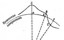



Zombie apocalypse play for two
New games about lego batman cars
Brief rules of chess How to play chess with yourself
How to make an enchantment table in minecraft and use it on a sword example
How to draw a skin for Minecraft yourself: a step by step description